Spatial data visualization

Setelah membaca chapter ini, pembaca diharapkan dapat:

• memvisualisasikan data meteorologi maritim pada peta spasial menggunakan Cartopy.

• mengintegrasikan data shapefile (batas wilayah pelayanan provinsi) menggunakan geopandas untuk analisis dan visualisasi data.

Intro

Plot peta spasial merupakan bagian fundamental dari analisis data meteorologi maritim. Peta spasial sangat berbeda dengan visualisasi data biasa karena:

• plot peta memerlukan proyeksi koordinat geografis dari 3d ke 2d,

• plot peta memerlukan dekorasi tambahan selain data yang akan diplot (seperti daratan, garis pantai, dst).

Pada chapter ini, kita akan memperlajari visualisasi peta secara spasial memanfaatkan library cartopy.

# load module

import cartopy
import cartopy.crs as ccrs

import xarray as xr
import pandas as pd
import matplotlib.pyplot as plt

Cartopy untuk visualisasi peta spasial

Cartopy dibangun dengan PROJ.4, numpy, shapely, dan matplotlib. Fitur utamanya terletak pada proyeksi berbasis class dengan kemampuan transformasi fitur geografis (line, polygon, dst).

ccrs.PlateCarree()

<cartopy.crs.PlateCarree object at 0x7fc34ab589e0>

Salah satu metode yang paling berguna yang ditambahkan oleh class di atas kelas Axes standar dari matplotlib adalah method coastlines. Tanpa argumen apa pun, metode ini akan menambahkan data garis pantai dari Natural Earth dengan skala 1:110.000.000 ke peta.

plt.figure(figsize=(10,5))
ax = plt.axes(projection=ccrs.PlateCarree())
ax.coastlines()

<cartopy.mpl.feature_artist.FeatureArtist at 0x7fc34a5b1950>

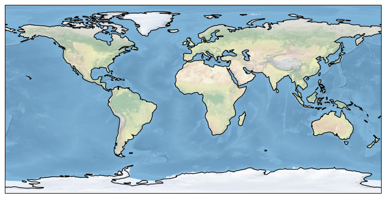
Kita juga bisa membuat subplot matplotlib dengan salah satu dari banyak pendekatan yang tersedia. Sebagai contoh, fungsi plt.subplots bisa digunakan:

fig, ax = plt.subplots(figsize=(10,5), subplot_kw={'projection':ccrs.PlateCarree()})
ax.stock_img()
ax.coastlines()

<cartopy.mpl.feature_artist.FeatureArtist at 0x7fc34a606350>

Regional map dan fitur

Plot peta regional dapat dilakukan menggunakan method .set_extent.

Beberapa fitur yang dapat ditambahkan kedalam map.

Fitur	Deskripsi
cartopy.features.BORDERS	Batas negara
cartopy.features.COASTLINE	Batas pantai
cartopy.feature.LAKES	Poligon danau
cartopy.feature.LAND	Poligon darat
cartopy.feature.OCEAN	Poligon laut
cartopy.feature.RIVERS	Line sungai

import cartopy.feature as cfeature
import numpy as np

coastline10 = cfeature.NaturalEarthFeature(category='physical', name='coastline', scale='10m')
land10 = cfeature.NaturalEarthFeature(category='physical', name='land', scale='10m')
plt.figure(figsize=(12, 6))
ax = plt.axes(projection=ccrs.PlateCarree())

extent = [90, 145, -12, 10]
ax.set_extent(extent)

ax.add_feature(cartopy.feature.OCEAN)
ax.add_feature(coastline10, edgecolor='black')
ax.add_feature(land10, facecolor='lightgrey', edgecolor='black')
ax.add_feature(cartopy.feature.BORDERS)
# ax.add_feature(cartopy.feature.LAKES, edgecolor='black')
# ax.add_feature(cartopy.feature.RIVERS)
ax.gridlines(draw_labels=True, dms=True, x_inline=False, y_inline=False)

<cartopy.mpl.gridliner.Gridliner at 0x7fc340c45f90>

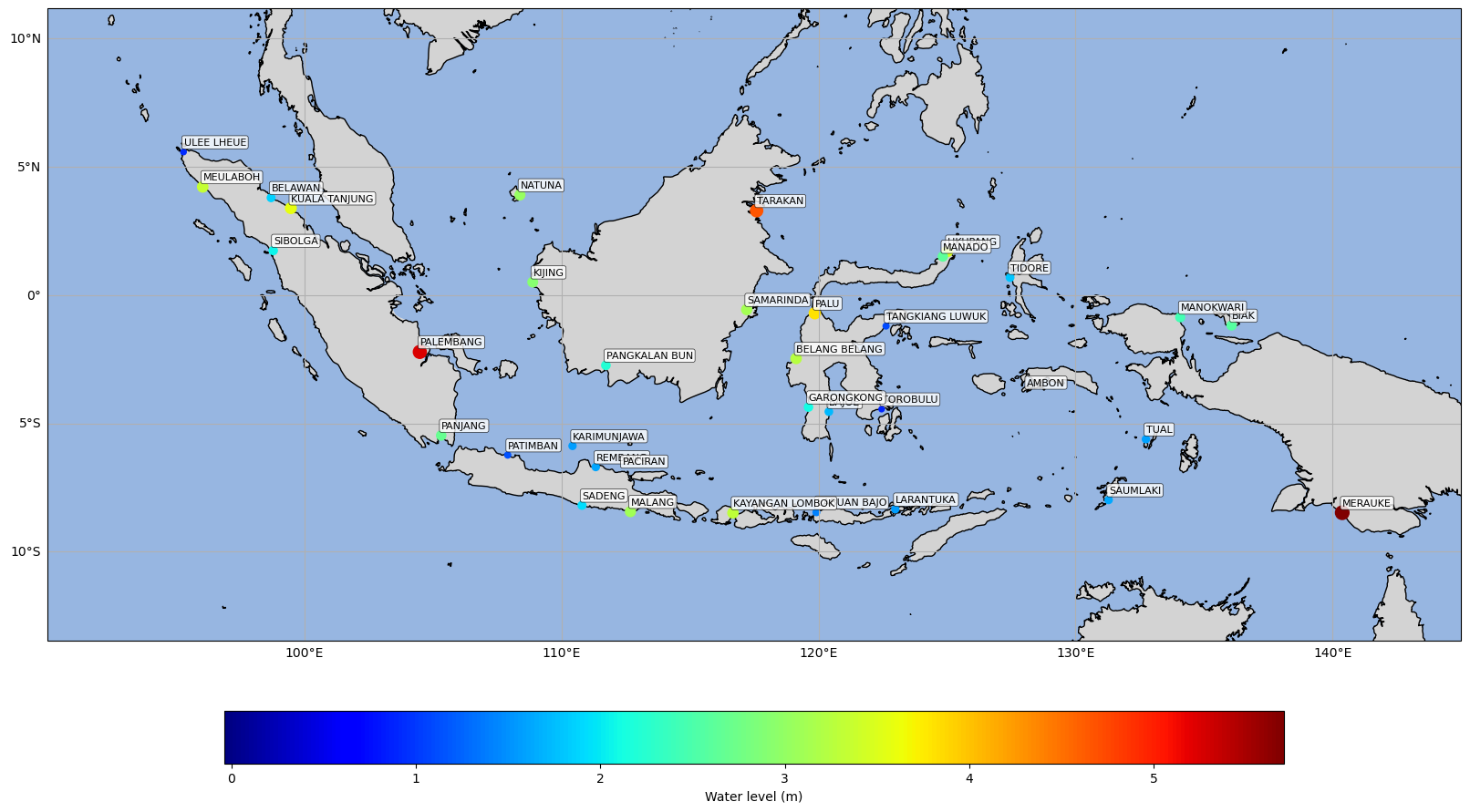
Plot data (1D)

Sampel data Marine Automatic Weather Station untuk Plot water level pada peta cartopy.

import pandas as pd

df = pd.read_csv("../data/sample_aws.csv").dropna().reset_index(drop=True)
display(df.head(3))
df.columns

	dat	wind_force_QC	wind_direction	lon	station_id	sunshine_total_QC	imei	sunshine_total_offset	tt_logger	water_sea_level_QC	...	wind_direction_QC	sea_surface_salinity_offset	wind_direction_offset	maximum_temperature_QC	wind_max_1h_QC	rr10	dew_point_temperature	battery_level_QC	bmkg_id	dew_point_temperature_offset
0	2025-01-01	1.0	208.60	111.728834	wigos_id:0-22000-0-5301768	1.0	300234068448940	0.0	27.0	1.0	...	1.0	0.0	-2.00	1.0	1.0	0.0	297.25	1.0	PBU	0.0
1	2025-01-01	1.0	211.77	136.076831	wigos_id:0-22000-0-5301795	1.0	300534061806700	0.0	27.0	1.0	...	1.0	0.0	-5.33	1.0	1.0	0.0	297.75	1.0	BIK	0.0
2	2025-01-01	1.0	204.80	117.206440	wigos_id:0-22000-0-5301785	1.0	300534061608660	0.0	27.0	1.0	...	1.0	0.0	-3.00	1.0	1.0	0.0	298.45	1.0	SMR	0.0

3 rows × 74 columns

Index(['dat', 'wind_force_QC', 'wind_direction', 'lon', 'station_id',
       'sunshine_total_QC', 'imei', 'sunshine_total_offset', 'tt_logger',
       'water_sea_level_QC', 'wind_force_offset', 'wl_radar',
       'minimum_temperature_offset', 'rr10_offset', 'tt_logger_QC',
       'wind_max_1h_direction', 'rr', 'wl_radar_QC', 'pressure', 'ph_sea_QC',
       'battery_level', 'sea_surface_salinity_QC', 'sea_temperature_offset',
       'ssr_sea_max', 'minimum_temperature', 'avg_relative_humidity_QC',
       'maximum_temperature', 'ssr_sea_QC', 'ssr_sea_offset',
       'tt_logger_offset', 'water_sea_level_offset', 'wl_radar_offset',
       'pressure_QC', 'process', 'ssr_sea', 'ph_sea', 'temperature_QC',
       'sunshine_total', 'wind_max_1h_direction_offset', 'temperature_offset',
       'sea_temperature_QC', 'temperature', 'rr_offset',
       'avg_relative_humidity_offset', 'wind_max_1h_offset', 'lat',
       'dew_point_temperature_QC', 'station_name', 'sea_temperature',
       'ssr_sea_max_QC', 'sea_surface_salinity', 'ssr_sea_max_offset',
       'wind_max_1h_direction_QC', 'ph_sea_offset', 'rr_QC',
       'minimum_temperature_QC', 'water_sea_level', 'pressure_offset',
       'wind_force', 'wind_max_1h', 'comm_type', 'avg_relative_humidity',
       'maximum_temperature_offset', 'rr10_QC', 'wind_direction_QC',
       'sea_surface_salinity_offset', 'wind_direction_offset',
       'maximum_temperature_QC', 'wind_max_1h_QC', 'rr10',
       'dew_point_temperature', 'battery_level_QC', 'bmkg_id',
       'dew_point_temperature_offset'],
      dtype='object')

dfsel = df[['water_sea_level', 'lon', 'lat', 'station_name']]
display(dfsel.head())

	water_sea_level	lon	lat	station_name
0	2.206	111.728834	-2.739063	PANGKALAN BUN
1	2.587	136.076831	-1.185679	BIAK
2	3.123	117.206440	-0.570467	SAMARINDA
3	5.240	104.488350	-2.217510	PALEMBANG
4	3.463	125.014493	1.698828	LIKUPANG

# axis initialization
fig, ax = plt.subplots(figsize=(20,20), dpi=100, subplot_kw={'projection':ccrs.PlateCarree()})

# cartopy features
extent = [90, 145, -12, 10]
ax.set_extent(extent)
ax.coastlines('10m')
ax.add_feature(cartopy.feature.OCEAN)
ax.add_feature(cartopy.feature.LAND, facecolor='lightgrey')

# plot data onto map
plot = ax.scatter(x=df['lon'], y=df['lat'], c=df['water_sea_level'], s=20*df['water_sea_level'], cmap='jet', zorder=2)
for _, row in df.iterrows():
    ax.text(row['lon']+0.01, row['lat']+0.2, row['station_name'],
            fontsize=8, ha='left', va='bottom', transform=ccrs.PlateCarree(),
                bbox=dict(
                facecolor='white',
                edgecolor='black',
                boxstyle='round,pad=0.2',
                linewidth=0.5,
                alpha=0.8
            )
    )

# add gridlines
gl = ax.gridlines(draw_labels=True, dms=True, x_inline=False, y_inline=False)
gl.top_labels = False
gl.right_labels = False

# add colorbar
plt.colorbar(plot, label='Water level (m)', shrink=0.75, orientation='horizontal', pad=0.05)
plt.show()

/opt/conda/envs/ofs/lib/python3.13/site-packages/matplotlib/collections.py:1008: RuntimeWarning: invalid value encountered in sqrt
  scale = np.sqrt(self._sizes) * dpi / 72.0 * self._factor

/opt/conda/envs/ofs/lib/python3.13/site-packages/matplotlib/collections.py:1008: RuntimeWarning: invalid value encountered in sqrt
  scale = np.sqrt(self._sizes) * dpi / 72.0 * self._factor
/opt/conda/envs/ofs/lib/python3.13/site-packages/matplotlib/collections.py:1008: RuntimeWarning: invalid value encountered in sqrt
  scale = np.sqrt(self._sizes) * dpi / 72.0 * self._factor

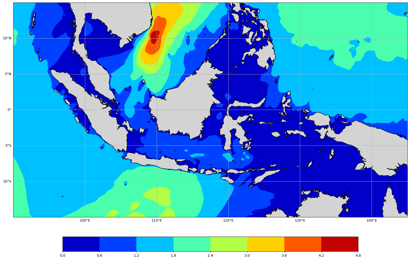
Plot data (2D)

Sampel data InaWaves hindcast untuk plot significant wave height di atas cartopy.

dset = xr.open_dataset("http://web.pusmar.id:8082/opendap/inawaves_hindcast/2025/H_hires_202501.nc")
dset

<xarray.Dataset> Size: 14GB
Dimensions:  (time: 249, lat: 481, lon: 881)
Coordinates:
  * time     (time) datetime64[ns] 2kB 2025-01-01 ... 2025-02-01
  * lat      (lat) float32 2kB -15.0 -14.94 -14.88 -14.81 ... 14.88 14.94 15.0
  * lon      (lon) float32 4kB 90.0 90.06 90.12 90.19 ... 144.9 144.9 145.0
Data variables: (12/17)
    hs       (time, lat, lon) float64 844MB ...
    hmax     (time, lat, lon) float64 844MB ...
    dir      (time, lat, lon) float64 844MB ...
    dp       (time, lat, lon) float64 844MB ...
    lm       (time, lat, lon) float64 844MB ...
    t01      (time, lat, lon) float64 844MB ...
    ...       ...
    ptp00    (time, lat, lon) float64 844MB ...
    ptp01    (time, lat, lon) float64 844MB ...
    ptp02    (time, lat, lon) float64 844MB ...
    pdi00    (time, lat, lon) float64 844MB ...
    pdi01    (time, lat, lon) float64 844MB ...
    pdi02    (time, lat, lon) float64 844MB ...
Attributes:
    source:       Inawaves - BMKG Ocean Forecast System (OFS)
    description:  Inawaves Model - Hindcast
    institution:  BMKG - Center For Marine Meteorology
    email:        produksi.maritim@bmkg.go.id
    Conventions:  CF-1.8

xarray.Dataset

• Dimensions:
  • time: 249
  • lat: 481
  • lon: 881
• Coordinates: (3)
  • time
    (time)
    datetime64[ns]
    2025-01-01 ... 2025-02-01

    long_name :

    Time

    standard_name :

    time

    array(['2025-01-01T00:00:00.000000000', '2025-01-01T03:00:00.000000000',
           '2025-01-01T06:00:00.000000000', ..., '2025-01-31T18:00:00.000000000',
           '2025-01-31T21:00:00.000000000', '2025-02-01T00:00:00.000000000'],
          shape=(249,), dtype='datetime64[ns]')

  • lat
    (lat)
    float32
    -15.0 -14.94 -14.88 ... 14.94 15.0

    long_name :

    Latitude

    standard_name :

    latitude

    units :

    degrees_north

    array([-15.    , -14.9375, -14.875 , ...,  14.875 ,  14.9375,  15.    ],
          shape=(481,), dtype=float32)

  • lon
    (lon)
    float32
    90.0 90.06 90.12 ... 144.9 145.0

    long_name :

    Longitude

    standard_name :

    longitude

    units :

    degrees_east

    array([ 90.    ,  90.0625,  90.125 , ..., 144.875 , 144.9375, 145.    ],
          shape=(881,), dtype=float32)

• Data variables: (17)
  • hs
    (time, lat, lon)
    float64
    ...

    long_name :

    Significant wave height

    standard_name :

    sea_surface_wave_significant_height

    units :

    m

    [105516489 values with dtype=float64]

  • hmax
    (time, lat, lon)
    float64
    ...

    long_name :

    Maximum Wave Height

    standard_name :

    sea_surface_wave_maximum_height

    units :

    m

    [105516489 values with dtype=float64]

  • dir
    (time, lat, lon)
    float64
    ...

    long_name :

    Mean Wave Direction

    standard_name :

    sea_surface_mean_wave_from_direction

    units :

    degree

    [105516489 values with dtype=float64]

  • dp
    (time, lat, lon)
    float64
    ...

    long_name :

    Peak Wave Direction

    standard_name :

    sea_surface_peak_wave_from_direction

    units :

    degree

    [105516489 values with dtype=float64]

  • lm
    (time, lat, lon)
    float64
    ...

    long_name :

    Wave Length

    standard_name :

    sea_surface_wave_mean_wavelength_from_variance_spectral_density_inverse_wavenumber_moment

    units :

    m

    [105516489 values with dtype=float64]

  • t01
    (time, lat, lon)
    float64
    ...

    long_name :

    Wave Period

    standard_name :

    sea_surface_wave_significant_period

    units :

    s

    [105516489 values with dtype=float64]

  • uwnd
    (time, lat, lon)
    float64
    ...

    long_name :

    Eastward Wind Speed

    standard_name :

    eastward_wind

    units :

    knot

    [105516489 values with dtype=float64]

  • vwnd
    (time, lat, lon)
    float64
    ...

    long_name :

    Northward Wind

    standard_name :

    northward_wind

    units :

    knot

    [105516489 values with dtype=float64]

  • phs00
    (time, lat, lon)
    float64
    ...

    long_name :

    Wind Sea Height

    standard_name :

    sea_surface_wind_wave_significant_height

    units :

    m

    [105516489 values with dtype=float64]

  • phs01
    (time, lat, lon)
    float64
    ...

    long_name :

    Primary Swell Height

    standard_name :

    sea_surface_primary_swell_wave_significant_height

    units :

    m

    [105516489 values with dtype=float64]

  • phs02
    (time, lat, lon)
    float64
    ...

    long_name :

    Secondary Swell Height

    standard_name :

    sea_surface_secondary_swell_wave_significant_height

    units :

    m

    [105516489 values with dtype=float64]

  • ptp00
    (time, lat, lon)
    float64
    ...

    long_name :

    Wind Sea Period

    standard_name :

    sea_surface_wind_wave_period

    units :

    s

    [105516489 values with dtype=float64]

  • ptp01
    (time, lat, lon)
    float64
    ...

    long_name :

    Primary Swell Period

    standard_name :

    sea_surface_primary_swell_wave_mean_period

    units :

    s

    [105516489 values with dtype=float64]

  • ptp02
    (time, lat, lon)
    float64
    ...

    long_name :

    Secondary Swell Period

    standard_name :

    sea_surface_secondary_swell_wave_mean_period

    units :

    s

    [105516489 values with dtype=float64]

  • pdi00
    (time, lat, lon)
    float64
    ...

    long_name :

    Wind Sea Direction

    standard_name :

    sea_surface_wind_wave_from_direction

    units :

    degree

    [105516489 values with dtype=float64]

  • pdi01
    (time, lat, lon)
    float64
    ...

    long_name :

    Primary Swell Direction

    standard_name :

    sea_surface_primary_swell_wave_from_direction

    units :

    degree

    [105516489 values with dtype=float64]

  • pdi02
    (time, lat, lon)
    float64
    ...

    long_name :

    Secondary Swell Direction

    standard_name :

    sea_surface_secondary_swell_wave_from_direction

    units :

    degree

    [105516489 values with dtype=float64]

• Indexes: (3)
  • time
    PandasIndex

    PandasIndex(DatetimeIndex(['2025-01-01 00:00:00', '2025-01-01 03:00:00',
                   '2025-01-01 06:00:00', '2025-01-01 09:00:00',
                   '2025-01-01 12:00:00', '2025-01-01 15:00:00',
                   '2025-01-01 18:00:00', '2025-01-01 21:00:00',
                   '2025-01-02 00:00:00', '2025-01-02 03:00:00',
                   ...
                   '2025-01-30 21:00:00', '2025-01-31 00:00:00',
                   '2025-01-31 03:00:00', '2025-01-31 06:00:00',
                   '2025-01-31 09:00:00', '2025-01-31 12:00:00',
                   '2025-01-31 15:00:00', '2025-01-31 18:00:00',
                   '2025-01-31 21:00:00', '2025-02-01 00:00:00'],
                  dtype='datetime64[ns]', name='time', length=249, freq=None))

  • lat
    PandasIndex

    PandasIndex(Index([   -15.0, -14.9375,  -14.875, -14.8125,   -14.75, -14.6875,  -14.625,
           -14.5625,    -14.5, -14.4375,
           ...
            14.4375,     14.5,  14.5625,   14.625,  14.6875,    14.75,  14.8125,
             14.875,  14.9375,     15.0],
          dtype='float32', name='lat', length=481))

  • lon
    PandasIndex

    PandasIndex(Index([    90.0,  90.0625,   90.125,  90.1875,    90.25,  90.3125,   90.375,
            90.4375,     90.5,  90.5625,
           ...
           144.4375,    144.5, 144.5625,  144.625, 144.6875,   144.75, 144.8125,
            144.875, 144.9375,    145.0],
          dtype='float32', name='lon', length=881))

• Attributes: (5)

  source :

  Inawaves - BMKG Ocean Forecast System (OFS)

  description :

  Inawaves Model - Hindcast

  institution :

  BMKG - Center For Marine Meteorology

  email :

  produksi.maritim@bmkg.go.id

  Conventions :

  CF-1.8

fig, ax = plt.subplots(figsize=(20,20), subplot_kw={'projection':ccrs.PlateCarree()})
extent = [90, 145, -12, 10]

ax.coastlines('10m')
ax.add_feature(cartopy.feature.LAND, facecolor='lightgrey', edgecolor='black')
mag = ax.contourf(dset.lon.data, dset.lat.data, dset.hs[0].data, cmap='jet', transform=ccrs.PlateCarree())
gl = ax.gridlines(draw_labels=True)
gl.top_labels = False
gl.right_labels = False

plt.colorbar(mag, shrink=.75, pad=0.05, orientation='horizontal')

<matplotlib.colorbar.Colorbar at 0x7fc336f57610>

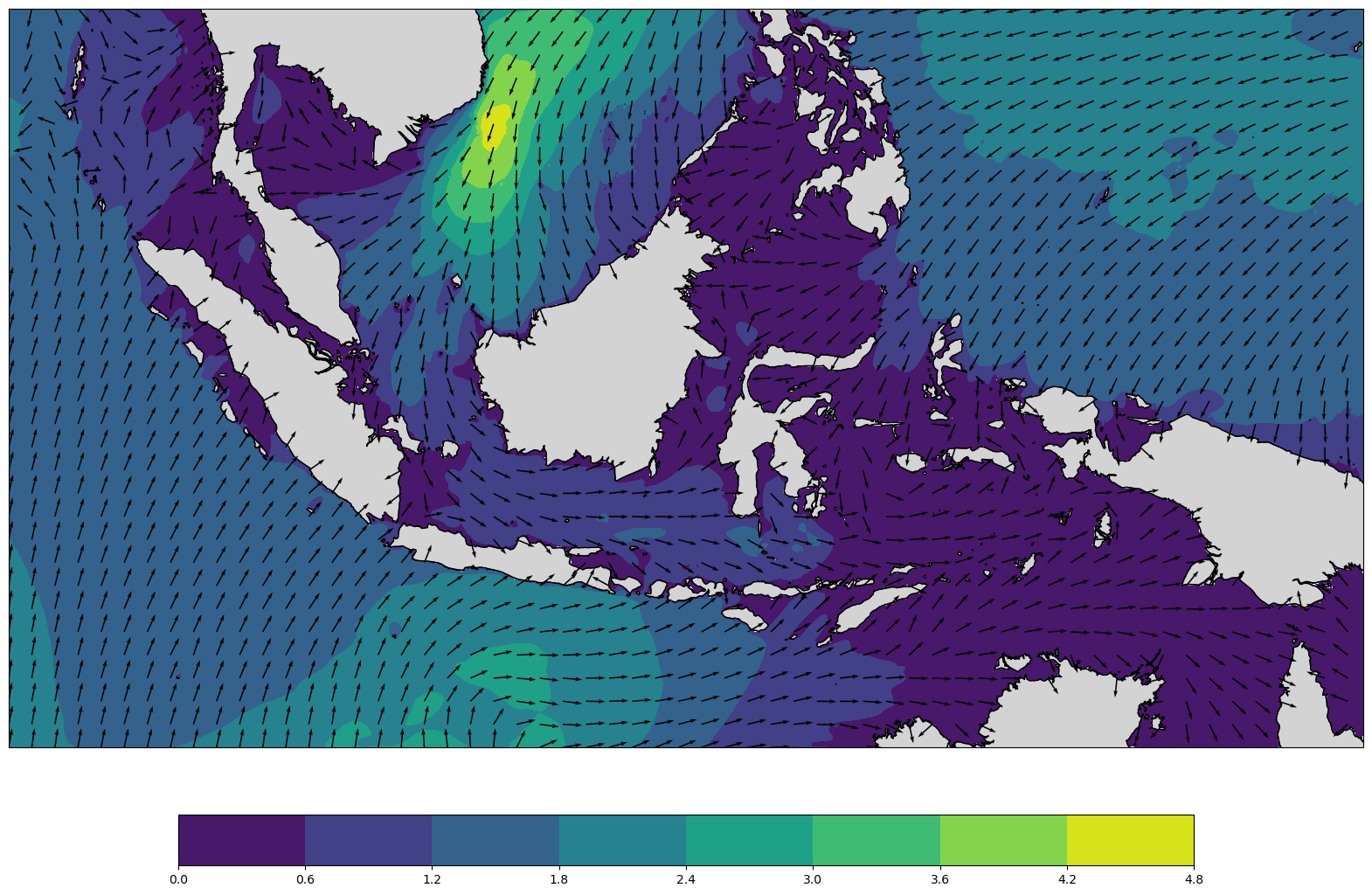
Menambahkan informasi arah gelombang menggunakan method .quiver.

Anatomi arrow di matplotlib.

lon = dset.lon.data
lat = dset.lat.data
data = dset.hs[0].data
uwave = np.cos(np.deg2rad(dset.dir[0].data))
vwave = np.sin(np.deg2rad(dset.dir[0].data))
arw_int = 15
arr_width = 0.001
arr_scale = 70 # length

fig, ax = plt.subplots(figsize=(20,20), subplot_kw={'projection':ccrs.PlateCarree()})
extent = [90, 145, -12, 10]

ax.coastlines('10m')
ax.add_feature(cartopy.feature.LAND, facecolor='lightgrey', edgecolor='black')
mag = ax.contourf(lon, lat, data, transform=ccrs.PlateCarree())
ax.quiver(
    lon[::arw_int], 
    lat[::arw_int], 
    uwave[::arw_int,::arw_int], 
    vwave[::arw_int,::arw_int],
    width=arr_width, 
    scale=arr_scale, 
    transform=ccrs.PlateCarree())

plt.colorbar(mag, shrink=.75, pad=0.05, orientation='horizontal')

<matplotlib.colorbar.Colorbar at 0x7fc335ced950>

💡 Worth to try: Cartopy

• Beberapa arow terlihat sampai menutupi wilayah darat, sesuaikan agar darat yang menutupi arrow. hint: gunakan argument zorder.

• Tambahkan fitur cartopy batas negara. hint: gunakan method .BORDER pada cartopy.feature.

• Tambahkan informasi seperti gridlines, judul peta, dan label colorbar.

• Coba untuk mengubah anatomi arrow, terlihat bahwa bagian head arrow proporsinya cukup kecil dibanding panjangnya. hint: gunakan argument .headwidth.

Layering shapefile

Data shapefile dapat dimanipulasi menggunakan library geopandas.

# load shapefile

import geopandas as gpd

shp = gpd.read_file("/data/local/shpmetoswilpro/METOS_WILPRO_20231018.shp")
shp.head(5)

	FID_METOS_	OBJECTID	DIS	Perairan	Met_Area	Label	ID	sub_ID	ID_MAR	ID_Stat	wilpro	geometry
0	34	1	1.0	None	Laut Arafuru bagian tengah	M	34	None	M. .34	None	None	POLYGON Z ((136.60373 -5.05887 0, 136.67687 -5...
1	16	1	1.0	None	Samudra Hindia selatan NTT	M	16	None	M. .16	None	None	POLYGON Z ((118.6756 -9.55198 0, 118.75928 -9....
2	43	1	1.0	None	Samudra Pasifik utara Papua	M	43	None	M. .43	None	None	POLYGON Z ((135.05306 -0.23913 0, 134.66088 -0...
3	2	1	1.0	None	Selat Malaka bagian tengah	M	02	None	M. .02	None	None	POLYGON Z ((101.0024 2.8619 0, 101.00152 2.862...
4	3	1	1.0	None	Samudra Hindia barat Aceh	M	03	None	M. .03	None	None	POLYGON Z ((94.85965 6.01528 0, 94.8417 5.9791...

shp.Met_Area.unique()

array(['Laut Arafuru bagian tengah', 'Samudra Hindia selatan NTT',
       'Samudra Pasifik utara Papua', 'Selat Malaka bagian tengah',
       'Samudra Hindia barat Aceh', 'Samudra Hindia barat Kep. Nias',
       'Samudra Hindia barat Kep. Mentawai',
       'Samudra Hindia barat Bengkulu', 'Laut Banda',
       'Samudra Hindia barat Lampung', 'Laut Maluku',
       'Samudra Hindia selatan Jawa Barat',
       'Samudra Hindia selatan Jawa Timur', 'Selat Malaka bagian utara',
       'Laut Natuna Utara', 'Laut Jawa bagian tengah',
       'Laut Jawa bagian timur', 'Laut Bali', 'Teluk Bone',
       'Selat Makassar bagian selatan', 'Laut Seram',
       'Laut Arafuru bagian Utara', 'Laut Flores',
       'Selat Karimata bagian selatan', 'Selat Karimata bagian utara',
       'Samudra Hindia selatan Banten',
       'Samudra Hindia selatan Jawa Tengah',
       'Samudra Hindia selatan DI Yogyakarta',
       'Samudra Hindia selatan Bali', 'Samudra Hindia selatan NTB',
       'Laut Jawa bagian barat', 'Laut Sumbawa',
       'Selat Makassar bagian utara', 'Selat Makassar bagian tengah',
       'Laut Sulawesi bagian timur', 'Laut Sulawesi bagian barat',
       'Laut Sulawesi bagian tengah', 'Samudra Pasifik utara Maluku',
       'Samudra Pasifik utara Papua Barat Daya',
       'Laut Arafuru bagian barat', 'Laut Arafuru bagian timur',
       'Selat Bali bagian utara', None,
       'Samudra Pasifik utara Papua Barat'], dtype=object)

type(shp)

geopandas.geodataframe.GeoDataFrame

shp.Label.unique()

array(['M', 'P'], dtype=object)

shp.Perairan.unique()

array([None, 'Aceh', 'Sumatra Utara', 'Riau', 'Sumatra Barat', 'Bengkulu',
       'Jambi', 'Sumatra Selatan', 'Jawa Barat', 'Jawa Tengah',
       'Kep. Riau', 'Kalimantan Barat', 'Kep. Bangka Belitung',
       'DKI Jakarta', 'Kalimantan Selatan', 'Kalimantan Utara',
       'Kalimantan Timur', 'Nusa Tenggara Barat', 'Nusa Tenggara Timur',
       'Gorontalo', 'Sulawesi Tengah', 'Sulawesi Selatan', 'Maluku Utara',
       'Sulawesi Utara', 'Papua', 'Papua Tengah', 'Papua Selatan',
       'DI Yogyakarta', 'Maluku', 'Sulawesi Barat', 'Kalimantan Tengah',
       'Jawa Timur', 'Banten', 'Lampung', 'Papua Barat Daya',
       'Papua Barat', 'Sulawesi Tenggara', 'Bali'], dtype=object)

Data shapefile di atas merupakan gabungan antara shp METOS (Met-Osean Area) yang dikelola oleh Pusat dan Wilpro (Wilayah Provinsi) yang dikelola oleh UPT. Dalam praktik ini, kita akan mencoba mengolah khusus untuk wilayah METOS.

Manipulasi tipe data geodataframe sepenuhnya identik dengan pandas DataFrame.

# Seleksi data untuk ilayah METOS berdasarkan kolom Label

shpmetos = shp[shp['Label'] == 'M']
shpmetos.head()

	FID_METOS_	OBJECTID	DIS	Perairan	Met_Area	Label	ID	sub_ID	ID_MAR	ID_Stat	wilpro	geometry
0	34	1	1.0	None	Laut Arafuru bagian tengah	M	34	None	M. .34	None	None	POLYGON Z ((136.60373 -5.05887 0, 136.67687 -5...
1	16	1	1.0	None	Samudra Hindia selatan NTT	M	16	None	M. .16	None	None	POLYGON Z ((118.6756 -9.55198 0, 118.75928 -9....
2	43	1	1.0	None	Samudra Pasifik utara Papua	M	43	None	M. .43	None	None	POLYGON Z ((135.05306 -0.23913 0, 134.66088 -0...
3	2	1	1.0	None	Selat Malaka bagian tengah	M	02	None	M. .02	None	None	POLYGON Z ((101.0024 2.8619 0, 101.00152 2.862...
4	3	1	1.0	None	Samudra Hindia barat Aceh	M	03	None	M. .03	None	None	POLYGON Z ((94.85965 6.01528 0, 94.8417 5.9791...

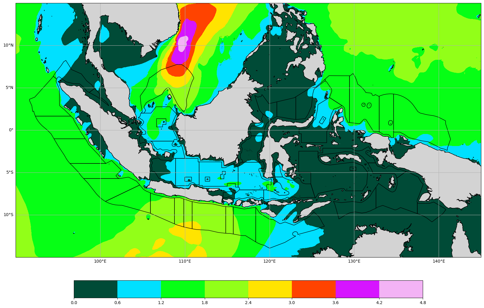
# LAYERING DI CARTOPY

fig, ax = plt.subplots(figsize=(20,20), subplot_kw={'projection':ccrs.PlateCarree()})
extent = [90, 145, -12, 10]

ax.coastlines('10m')
ax.add_feature(cartopy.feature.LAND, facecolor='lightgrey', edgecolor='black')
mag = ax.contourf(dset.lon.data, dset.lat.data, dset.hs[0].data, cmap='gist_ncar', transform=ccrs.PlateCarree())
shpmetos.plot(ax=ax, facecolor='none', edgecolor='black', linewidth=1, transform=ccrs.PlateCarree())

gl = ax.gridlines(draw_labels=True)
gl.top_labels = False
gl.right_labels = False

plt.colorbar(mag, shrink=.75, pad=0.05, orientation='horizontal')

<matplotlib.colorbar.Colorbar at 0x7fc335ac6fd0>

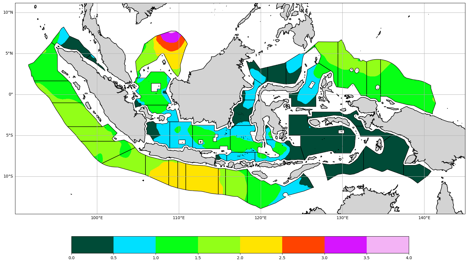
Clipping dapat dilakukan dengan bantuan module rioxarray.

import rioxarray

shpmetos = shpmetos.to_crs("EPSG:4326")

clipped = dset.hs[0].rio.write_crs("EPSG:4326").rio.clip(shpmetos.geometry, shpmetos.crs, drop=True)

fig, ax = plt.subplots(figsize=(20, 20), subplot_kw={'projection': ccrs.PlateCarree()})
ax.set_extent([90, 145, -13, 10])
ax.coastlines('10m')
ax.add_feature(cartopy.feature.LAND, facecolor='lightgrey', edgecolor='black')

mag = ax.contourf(clipped.lon.data, clipped.lat.data, clipped.data, cmap='gist_ncar', transform=ccrs.PlateCarree())

shpmetos.plot(ax=ax, facecolor='none', edgecolor='black', linewidth=1, transform=ccrs.PlateCarree())

gl = ax.gridlines(draw_labels=True)
gl.top_labels = False
gl.right_labels = False

plt.colorbar(mag, shrink=.75, pad=0.05, orientation='horizontal')

<matplotlib.colorbar.Colorbar at 0x7fc3358a9f90>

💡 Worth to try: Wilayah Provinsi

1. Buat Peta serupa untuk wilayah Provinsi masing-masing peserta berasal (UPT).

Hint: Buat seleksi Geodataframe berdasarkan Kolom Perairan. Contoh:

shpaceh = shp[shp['Perairan'] == 'Aceh']

2. Plot juga perlu ditambahkan informasi judul dan label colorbar

3. Coba juga untuk memplot arah gelombang menggunakan .quiver

# Your script here