Python scientific libraries#
Setelah membaca ini, pembaca diharapkan dapat memahami penggunaan library NumPy, Pandas, dan Matplotlib untuk pengolahan data.
Mengapa menggunakan libraries?#
Library diperlukan untuk memudahkan pemrosesan data sesuai dengan fokus spesifik yang diperlukan.
Library python yang umum digunakan dalam pengolahan data meteorologi maritim.
No |
Library |
Penggunaan |
|---|---|---|
1 |
NumPy |
Manipulasi array |
2 |
Pandas |
manipulasi data tabular |
3 |
Matplotlib |
visualisasi data |
—Tidak disampaikan dalam Mata Pelatihan 1, namun di Mata Pelatihan 2— |
||
4 |
Xarray |
manipulasi data multidimensi |
5 |
Cartopy |
visualisasi map |
6 |
Geopandas |
manipulasi data geospasial |
NumPy#
NumPy menyediakan dukungan untuk array, yang lebih efisien dan praktis daripada list Python untuk data numerik.
Konsep: Membuat array, atribut array, operasi array dasar.
# Mengimport library
import numpy as np
Creating NumPy array#
# Create a one-dimensional array of integer
arr = np.array([1,2,3,4,5])
print(arr

# Create a 2D array of floats
arr = np.array([[1.1, 2.3],[3.1,4.2]])
print(arr)
  Cell In[2], line 3
    print(arr
         ^
SyntaxError: '(' was never closed
Indexing#
# Indexing
# Create a 2D array
arr = np.aray([[1,2,3],[4,5,6],[7,8,9]])
print(arr)
[[1 2 3]
 [4 5 6]
 [7 8 9]]
# Access the element in the first row, second column
selected = arr[0,1]
print(selected)
2
Slicing#
# Slicing
# Create 1D array
arr = np.arange(10)
print(arr)

# Access the FIRST 5 elements
print(arr:5])

# Access the LAST 5 elements
print(arr[-5:])

# Access elements having even index
print(arr[::2])
[0 1 2 3 4 5 6 7 8 9]
[0 1 2 3 4]
[5 6 7 8 9]
[0 2 4 6 8]
Math operations#
# Mathematical Operations
# Create 1D array
arr = np.array([1,2,3,4,5])
print(arr)

# Operation of adding the value of each element
print(arr2)

# Operation of multiplication of each element
print(arr*3)

# Compute dot products of the array with itself
print(np.dot(arr,arr))
[1 2 3 4 5]
[3 4 5 6 7]
[ 3  6  9 12 15]
55
Aggregation#
# Aggregation Operations
# Create 1D array
arr = np.array([1,2,3,4,5])
print(arr)

# Finding max value
print(np.maxarr))

# Finding min value
print(np.min(arr))

# Finding standard deviation
print(np.std(arr))
[1 2 3 4 5]
5
1
1.4142135623730951
Reshaping and Transposing#
# Create 1D array
arr = np.array([1,2,3,4,5,6])
print(arr)

# Reshape the array into a 2D array
result = arr.reshape(2,3)
print(result)

# Transpose array
print(result.T)
[1 2 3 4 5 6]
[[1 2 3]
 [4 5 6]]
[[1 4]
 [2 5]
 [3 6]]
Pandas#
# Mengimport library
import padas as pd
Series#
Series adalah struktur data 1 dimensi seperti array atau list, tetapi memiliki index.
# Create a Series
s = pd.Series(
    [1, 3, 5, np.nan, 6, 8]
)
print(s)
0    1.0
1    3.0
2    5.0
3    NaN
4    6.0
5    8.0
dtype: float64
DataFrame#
DataFrame adalah struktur data 2 dimensi, seperti tabel Excel.
# Membuat dataframe
data = {'temp': [27,30,29]
        'rh': [70,75,80],
        'wx': ['clear','cloudy','rain']}

df = pd.DataFrame(data,index=['Jakarta','Tokyo','NewYork'])
df
| temp | rh | wx | |
|---|---|---|---|
| Jakarta | 27 | 70 | clear |
| Tokyo | 30 | 75 | cloudy |
| NewYork | 29 | 80 | rain |
print(df)
         temp  rh      wx
Jakarta    27  70   clear
Tokyo      30  75  cloudy
NewYork    29  80    rain
df.describe()
| temp | rh | |
|---|---|---|
| count | 3.000000 | 3.0 |
| mean | 28.666667 | 75.0 |
| std | 1.527525 | 5.0 |
| min | 27.000000 | 70.0 |
| 25% | 28.000000 | 72.5 |
| 50% | 29.000000 | 75.0 |
| 75% | 29.500000 | 77.5 |
| max | 30.000000 | 80.0 |
Indexing & Slicing#
Mengakses Kolom#
df['temp'] # atau df.temp
Jakarta    27
Tokyo      30
NewYork    29
Name: temp, dtype: int64
Mengakses Baris dengan Label (.loc)#
df.loc['Tokyo']
temp        30
rh          75
wx      cloudy
Name: Tokyo, dtype: object
df.loc[['Tokyo', 'NewYork']]
| temp | rh | wx | |
|---|---|---|---|
| Tokyo | 30 | 75 | cloudy |
| NewYork | 29 | 80 | rain |
Mengakses Baris dengan Posisi (.iloc)#
# mengakses baris posisi ke 0
df.iloc[0]
temp       27
rh         70
wx      clear
Name: Jakarta, dtype: object
# mengakses baris posisi ke 1 sampai 2
df.iloc[1:3]
| temp | rh | wx | |
|---|---|---|---|
| Tokyo | 30 | 75 | cloudy |
| NewYork | 29 | 80 | rain |
Mengakses Sel Tertentu (Baris & Kolom Sekaligus)#
# mengakses nilai temp di baris Jakarta.
df.loc['Jakarta', 'temp']
np.int64(27)
# mengakses nilai rh di baris ke-2 (NewYork).
df.iloc[2, 1]
np.int64(80)
Slicing Kolom dan Baris Sekaligus#
# Mengakses subset baris dari Tokyo sampai NewYork dan kolom dari temp sampai rh.
df.loc['Tokyo':'NewYork', 'temp':'rh']
| temp | rh | |
|---|---|---|
| Tokyo | 30 | 75 |
| NewYork | 29 | 80 |
Filtering#
# Menampilkan kota-kota dengan suhu (temp) lebih dari 28°C.
df[df['temp'] > 28]
| temp | rh | wx | |
|---|---|---|---|
| Tokyo | 30 | 75 | cloudy |
| NewYork | 29 | 80 | rain |
Math operations#
comfort_index = 0.5*(df['temp']+df['rh'])
df['comfort_index'] = comfort_index
df
| temp | rh | wx | comfort_index | |
|---|---|---|---|---|
| Jakarta | 27 | 70 | clear | 48.5 |
| Tokyo | 30 | 75 | cloudy | 52.5 |
| NewYork | 29 | 80 | rain | 54.5 |
df.loc['Jakarta', 'temp'] += 2
df.loc['Tokyo', 'temp'] -= 2
df
| temp | rh | wx | comfort_index | |
|---|---|---|---|---|
| Jakarta | 29 | 70 | clear | 48.5 |
| Tokyo | 28 | 75 | cloudy | 52.5 |
| NewYork | 29 | 80 | rain | 54.5 |
Agregasi#
RHmin = df['rh'].min()
RHmean = df['rh'].mean()
RHmax = df['rh'].max()
RHQ1 = df['rh'].quantile(0.25)
RHQ3 = df['rh'].quantile(0.75)
print(RHmin,RHmean,RHmax,RHQ1,RHQ3)
70 75.0 80 72.5 77.5
💡 WORTH TO TRY: Numpy x Pandas#
Buatlah sebuah dataframe berisi 2 kolom: bilangan ganjil 1 - 100 dan bilangan genap 1 - 100.
Buatlah 1 kolom baru berisi hasil perhitungan 2*(elemen ganjil + elemen genap)
Buatlah 1 kolom baru berisi Boolean untuk menandakan apakah bilangan ganjil di baris yang sama bilangan prima. Hint: buat fungsi dan gunakan pandas apply method
Matplotlib#
matplotlib adalah library visualisasi data yang paling umum digunakan di Python. Modul utamanya adalah pyplot, yang sering diimpor sebagai plt.
import matplotlib.pyplot as plt
Membuat Plot Sederhana#
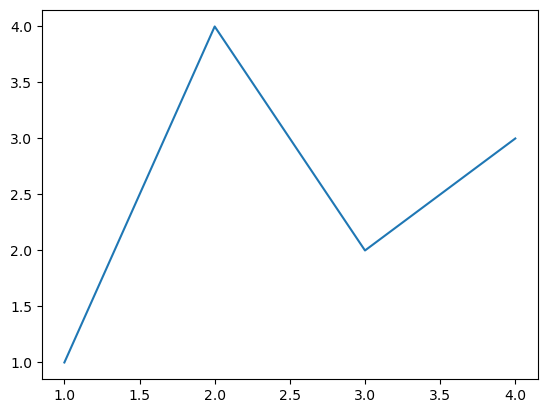
Gunakan plt.subplots() untuk membuat figure dan axes, kemudian gunakan .plot() untuk menggambar data.
# Mengimport library
import matplotlib.pyplot as plt

fig, ax = plt.subplots()             # Create a figure containing a single Axes.
ax.plot([1, 2, 3, 4], [1, 4, 2, 3])  # Plot some data on the Axes.
plt.show()                           # Show the figure.
Anatomy dari Figure#
Setiap plot terdiri dari komponen:
Figure: kanvas utama
Axes: area plot
Title: judul plot (
ax.set_title)X & Y label: nama sumbu (
ax.set_xlabel,ax.set_ylabel)Legend, Grid, Spines, Ticks, dll.
📌 Lihat gambar berikut untuk referensi visual:

Mengatur Ukuran dan Tata Letak Figure#
Gunakan figsize=(lebar, tinggi) saat membuat figure.
fig = plt.figure()
plt.show()
<Figure size 640x480 with 0 Axes>
fig = plt.figure(figsize=(13,5))
<Figure size 1300x500 with 0 Axes>
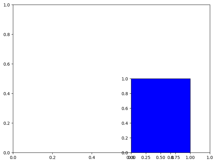
Menambahkan Beberapa Axes#
Gunakan fig.add_axes() untuk menambahkan beberapa panel secara bebas.
np.linspace(0, 100, 11)
np.zeros((2, 1), int)

fig = plt.figure()
ax = fig.add_axes([0,0,1,1])
fig = plt.figure()
ax1 = fig.add_axes([0,0,1,1])
ax2 = fig.add_axes([0.6,0,0.3,0.5], facecolor='b')
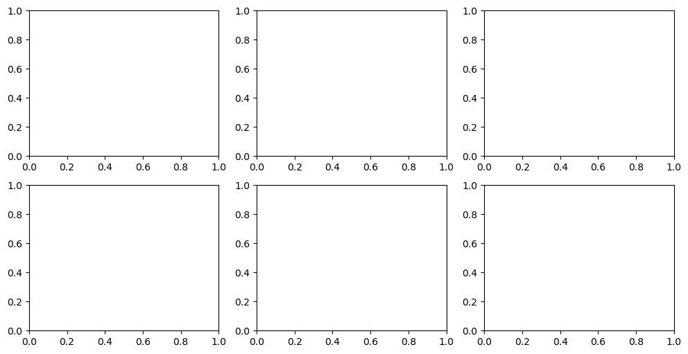
Subplots: Beberapa Grafik dalam Satu Gambar#
Gunakan plt.subplots(nrows, ncols) untuk membuat grid plot otomatis.
fig = plt.figure(figsize=(12,6))
axes = fig.subplots(nrows=2, ncols=3)
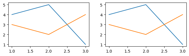
fig,ax = plt.subplots(figsize=(8,2), nrows=1, ncols=2)
ax[0].plot([1,2,3],[4,5,1]
ax[0].plot([1,2,3],[3,2,4])
ax[1].plot([1,2,3],[4,5,1])
ax[1].plot([1,2,3],[3,2,4])
plt.show()
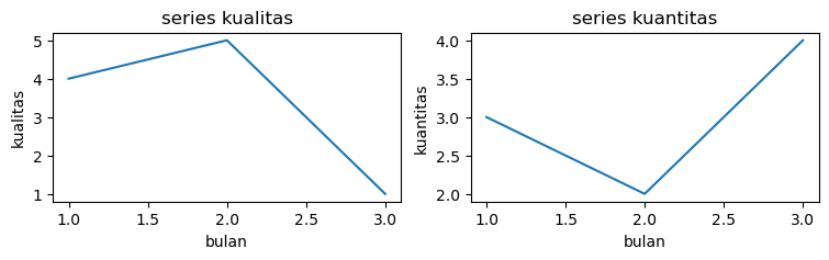
Menambahkan Label, Judul, dan Anotasi#
fig,ax = plt.subplots(figsize=(9,2),ncols=2)
ax0,ax1 = ax

ax0.plot([1,2,3],[4,5,1])
ax0.set_xlabel('bulan')
ax0.set_ylabe('kualitas')
ax0.set_title('series kualitas')

ax1.plot([1,2,3],[3,2,4])
ax1.set_xlabel('bulan')
ax1.set_ylabel('kuantitas')
ax1.set_title('series kuantitas')

plt.show()
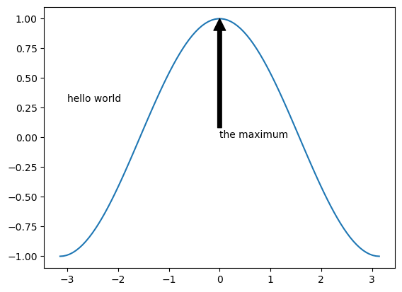
import numpy as np
x = np.linspace(-np.pi, np.pi, 100)
y = np.cos(x)
z = np.sin(6*x)

fig, ax = plt.subplots()
ax.plot(x, y)
ax.text(-3, 0.3, 'hello world')
ax.annotate('the maximum', xy=(0, 1),
             xytext=(0, 0), arrowprops={'facecolor': 'k'})
Text(0, 0, 'the maximum')
E. Tips#
1. Memanggil method yang tersimpan dalam library#
Method dapat dipanggil dengan menambahkan . kemudian tab keyboard.

***
np.
2. Mendapatkan bantuan#
Bantuan menggunakan command help atau ?.
help(np.array)
Help on built-in function array in module numpy:

array(...)
    array(object, dtype=None, *, copy=True, order='K', subok=False, ndmin=0,
          like=None)

    Create an array.

    Parameters
    ----------
    object : array_like
        An array, any object exposing the array interface, an object whose
        ``__array__`` method returns an array, or any (nested) sequence.
        If object is a scalar, a 0-dimensional array containing object is
        returned.
    dtype : data-type, optional
        The desired data-type for the array. If not given, NumPy will try to use
        a default ``dtype`` that can represent the values (by applying promotion
        rules when necessary.)
    copy : bool, optional
        If ``True`` (default), then the array data is copied. If ``None``,
        a copy will only be made if ``__array__`` returns a copy, if obj is
        a nested sequence, or if a copy is needed to satisfy any of the other
        requirements (``dtype``, ``order``, etc.). Note that any copy of
        the data is shallow, i.e., for arrays with object dtype, the new
        array will point to the same objects. See Examples for `ndarray.copy`.
        For ``False`` it raises a ``ValueError`` if a copy cannot be avoided.
        Default: ``True``.
    order : {'K', 'A', 'C', 'F'}, optional
        Specify the memory layout of the array. If object is not an array, the
        newly created array will be in C order (row major) unless 'F' is
        specified, in which case it will be in Fortran order (column major).
        If object is an array the following holds.

        ===== ========= ===================================================
        order  no copy                     copy=True
        ===== ========= ===================================================
        'K'   unchanged F & C order preserved, otherwise most similar order
        'A'   unchanged F order if input is F and not C, otherwise C order
        'C'   C order   C order
        'F'   F order   F order
        ===== ========= ===================================================

        When ``copy=None`` and a copy is made for other reasons, the result is
        the same as if ``copy=True``, with some exceptions for 'A', see the
        Notes section. The default order is 'K'.
    subok : bool, optional
        If True, then sub-classes will be passed-through, otherwise
        the returned array will be forced to be a base-class array (default).
    ndmin : int, optional
        Specifies the minimum number of dimensions that the resulting
        array should have.  Ones will be prepended to the shape as
        needed to meet this requirement.
    like : array_like, optional
        Reference object to allow the creation of arrays which are not
        NumPy arrays. If an array-like passed in as ``like`` supports
        the ``__array_function__`` protocol, the result will be defined
        by it. In this case, it ensures the creation of an array object
        compatible with that passed in via this argument.

        .. versionadded:: 1.20.0

    Returns
    -------
    out : ndarray
        An array object satisfying the specified requirements.

    See Also
    --------
    empty_like : Return an empty array with shape and type of input.
    ones_like : Return an array of ones with shape and type of input.
    zeros_like : Return an array of zeros with shape and type of input.
    full_like : Return a new array with shape of input filled with value.
    empty : Return a new uninitialized array.
    ones : Return a new array setting values to one.
    zeros : Return a new array setting values to zero.
    full : Return a new array of given shape filled with value.
    copy: Return an array copy of the given object.


    Notes
    -----
    When order is 'A' and ``object`` is an array in neither 'C' nor 'F' order,
    and a copy is forced by a change in dtype, then the order of the result is
    not necessarily 'C' as expected. This is likely a bug.

    Examples
    --------
    >>> import numpy as np
    >>> np.array([1, 2, 3])
    array([1, 2, 3])

    Upcasting:

    >>> np.array([1, 2, 3.0])
    array([ 1.,  2.,  3.])

    More than one dimension:

    >>> np.array([[1, 2], [3, 4]])
    array([[1, 2],
           [3, 4]])

    Minimum dimensions 2:

    >>> np.array([1, 2, 3], ndmin=2)
    array([[1, 2, 3]])

    Type provided:

    >>> np.array([1, 2, 3], dtype=complex)
    array([ 1.+0.j,  2.+0.j,  3.+0.j])

    Data-type consisting of more than one element:

    >>> x = np.array([(1,2),(3,4)],dtype=[('a','<i4'),('b','<i4')])
    >>> x['a']
    array([1, 3], dtype=int32)

    Creating an array from sub-classes:

    >>> np.array(np.asmatrix('1 2; 3 4'))
    array([[1, 2],
           [3, 4]])

    >>> np.array(np.asmatrix('1 2; 3 4'), subok=True)
    matrix([[1, 2],
            [3, 4]])
# atau menggunakan ?
np?
Type:        module
String form: <module 'numpy' from '/home/tyo/miniconda3/envs/ofs/lib/python3.13/site-packages/numpy/__init__.py'>
File:        ~/miniconda3/envs/ofs/lib/python3.13/site-packages/numpy/__init__.py
Docstring:
NumPy
=====

Provides
  1. An array object of arbitrary homogeneous items
  2. Fast mathematical operations over arrays
  3. Linear Algebra, Fourier Transforms, Random Number Generation

How to use the documentation
----------------------------
Documentation is available in two forms: docstrings provided
with the code, and a loose standing reference guide, available from
`the NumPy homepage <https://numpy.org>`_.

We recommend exploring the docstrings using
`IPython <https://ipython.org>`_, an advanced Python shell with
TAB-completion and introspection capabilities.  See below for further
instructions.

The docstring examples assume that `numpy` has been imported as ``np``::

  >>> import numpy as np

Code snippets are indicated by three greater-than signs::

  >>> x = 42
  >>> x = x + 1

Use the built-in ``help`` function to view a function's docstring::

  >>> help(np.sort)
  ... # doctest: +SKIP

For some objects, ``np.info(obj)`` may provide additional help.  This is
particularly true if you see the line "Help on ufunc object:" at the top
of the help() page.  Ufuncs are implemented in C, not Python, for speed.
The native Python help() does not know how to view their help, but our
np.info() function does.

Available subpackages
---------------------
lib
    Basic functions used by several sub-packages.
random
    Core Random Tools
linalg
    Core Linear Algebra Tools
fft
    Core FFT routines
polynomial
    Polynomial tools
testing
    NumPy testing tools
distutils
    Enhancements to distutils with support for
    Fortran compilers support and more (for Python <= 3.11)

Utilities
---------
test
    Run numpy unittests
show_config
    Show numpy build configuration
__version__
    NumPy version string

Viewing documentation using IPython
-----------------------------------

Start IPython and import `numpy` usually under the alias ``np``: `import
numpy as np`.  Then, directly past or use the ``%cpaste`` magic to paste
examples into the shell.  To see which functions are available in `numpy`,
type ``np.<TAB>`` (where ``<TAB>`` refers to the TAB key), or use
``np.*cos*?<ENTER>`` (where ``<ENTER>`` refers to the ENTER key) to narrow
down the list.  To view the docstring for a function, use
``np.cos?<ENTER>`` (to view the docstring) and ``np.cos??<ENTER>`` (to view
the source code).

Copies vs. in-place operation
-----------------------------
Most of the functions in `numpy` return a copy of the array argument
(e.g., `np.sort`).  In-place versions of these functions are often
available as array methods, i.e. ``x = np.array([1,2,3]); x.sort()``.
Exceptions to this rule are documented.